Monthly Archives: August 2013

Stefan's equation for sea ice thickness

Arctic Ice 2, Wikimedia Commons

Arctic Ice 2, Wikimedia Commons

Let's get to it! Today's worksheet is about deriving Stefan's equation. In 1891 Josef Stefan came up with a simple model for the thickness of sea ice, using thermodynamic reasoning and the data from British and German Arctic explorers. We, too, can trace through the thermodynamic reasoning. I found it harder to find straightforward sea ice thickness data for areas without snow.

To get technical here, we can start with the heat equation and some boundary conditions on the temperature at the top of the slab of sea ice and the bottom of the slab of sea ice. It's easiest to assume, though, that temperature in the ice sheet depends on vertical depth from the top of the ice sheet -- not so much on horizontal coordinates. That means we can use a model with one spatial dimension, depth . Then a reasonable simplification of the heat equation tells us that temperature depends on depth and time in the following way:
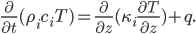
Continue reading

Momentary interlude

Check out this beautiful visualization of seasonal land ice and vegetation variation at NPR or at the original source:

Breathing earth

Breathing earth

Sea ice: a very baby model

I was traveling last week for a delightful conference on quantum cohomology, affine Schubert calculus, and the Peterson isomorphism. Crazy stuff. I had somehow expected to post during that -- but I learned something, which is that posting does not happen during intense conferences. I'll deal with that differently next time!

Many weeks ago in a discussion on LinkedIn someone suggested I write a post on sea ice, and I've been reading about sea ice ever since. It is complicated! Sea ice is the ice in the polar regions that floats on the sea, of course. It plays a huge role in climate because of its reflectivity, and we watch the growth and shrinkage of sea ice to monitor the state of the Arctic and Antarctic. But sea ice isn't just ice like an ice cube. Because the sea is salty, and salty water and fresh water freeze at different temperatures, there are some complicated phenomena that go on.

In the sea ice there are polynyas, areas of open water on top of the ice, and brine channels filled with bacteria and other little creatures. The ice itself ranges from new ice, starting with frazil ice through nilas ice through the stuff we think of when we think "ice." Even the names are exotic. Check out this picture below from the Advanced Land Imager (ALI) on NASA’s Earth Observing-1 (EO-1) satellite:

satellite photo of sea ice

Zoom in to see labels for frazil and nilas.

One of the sites I'm using for a resource for the coming worksheet has a lot more cool pictures, so check it out.

With all this complexity in biology, climate, physics, and thermodynamics, there's a bit of work involved in simplifying the models for a calculus worksheet. The worksheet will get done by Thursday and will focus on Stefan's model (from 1890!) for the thickness of sea ice. It will use a bit of integration and some differential equations.

Assumptions need to be made to produce a model this simple: I'm going to assume no snow on top of my ice, no brine channels or microorganisms messing up my idealized slab, a linear temperature gradient inside the ice. Even with these assumptions we can make rough predictions about how sea ice thickness evolves.

But, so that I don't leave you without any classroom resource today, I leave you with a link to a nice precalculus activity on modeling ice thickness. I just discovered Plus Magazine, the source, today. It's a nice place to look for short articles on beautiful mathematics!

Our leaky atmosphere

Backing away from the sensational headlines of last week, here's something a bit more relaxing. Our atmosphere is leaking away into space and maybe someday eventually we won't have one anymore. How's that?

Alright. I exaggerate a bit here -- the force of gravity is enough to keep nitrogen and oxygen around, as well as lovely greenhouse gases like carbon dioxide and methane. These are heavy molecules! Hydrogen, on the other hand, is really light. It reaches escape velocity fairly easily, especially at the outer reaches of the earth's atmosphere.

For a more nuanced look at atmospheric escape, check out the Scientific American article. I'm linking to an author's website because I can't get this article at the Scientific American site even via Cornell's library.

Today's worksheet is another longish one. I might consider splitting it up. The first two pages guide the student through a derivation of escape velocity using the chain rule, integration, and limits. It's one of those activities that dredges up everything a student had to learn all semester, yet in the end none of the integration or limits are that hard. The last page (the third) asks some very concrete questions about the escape velocity for hydrogen molecules, relating this velocity to temperature. "Is it hot enough for hydrogen to escape?" is the main question.

I have to confess that I spent all day traveling to a math conference and I'm a bit underslept. As I went through my calculations I realized that hydrogen could escape from anywhere in the earth's atmosphere, and this really alarmed me! We are all going to perish! until I realized that indeed that's the case, and that's why we basically have no hydrogen in our atmosphere. It's ok. Can't breathe that stuff anyway.

Let me know if you use this worksheet and whether you think it would be better broken up into parts. I like the surprising results, and I like the fact that it brings together the chain rule, integration, and limits. It would be fun to extend it and talk about the moon's lack of atmosphere and Venus's crushing anvil of an atmosphere. We sometimes take for granted our Goldilocks world...

Calc Roundup: Atmospheric Escape

Drinking drugs in Denver

How's that for a sensational headline?

This post is a bit late because of units. I got some wonderful data on personal care products and pharmaceuticals in wastewater from a reader: several pages of information on what's going into and coming out of the wastewater treatment plants in Silverthorne, Dillon, and Frisco, Colorado. These three wastewater treatment plants treat water from homes all around the Dillon Reservoir and then put treated water out into the reservoir itself, which eventually provides drinking water to Denver. They're doing the same great work wastewater treatment plants around the US and the world are doing: taking our extra coffee, our dishwater, and our waste and putting out pretty clean water!

The study I'm looking at used six trips over three years to look at influent (incoming water) and effluent (outgoing water) at these wastewater treatment sites. The authors used grab samples -- quick samples taken at one time, rather than samples taken at specific repeated times or water sampled throughout the day -- to get a cost effective test of water quality. Now, water spends some time in the wastewater treatment plant (this is called resonance time or residence time) and so a grab sample will not reflect what happens to a particular batch of water that goes in -- if it takes three hours, for instance, for water to get processed, but you take samples of influent and effluent ten minutes apart, you're measuring different parts of the stream. That will explain a bit of the weirdness we encounter on page three of the worksheet. Naproxen and cocaine are very effectively removed from water by current treatments, but hydrocodone is not and so it looks like more is coming out of the treatment plant than is going in!

Back to units, though: I wanted to do a worksheet using Riemann sums to estimate quantities of pharmaceuticals in the water supply, but all my data is in nanograms per liter and I wanted to look at it against time rather than volume. So I had to figure out how to get nanograms or grams per day, and that involved finding out how much water each wastewater treatment plant processed. Not totally easy. But I did manage it roughly. I found that in 2002-2004 the Snake River Wastewater Treatment plant was processing about 27% of its official capacity of 2.6 million gallons per day and used that figure. The Joint Sewer Authority (JSA) plant in Silverthorne says in its financial statement that it processes four million gallons/day. (I'd like to check those numbers, and have an email out to the Snake River folks.) Turn those into liters, and we can get nanograms per day. But those numbers are ugly decimals, so let's talk about grams per day!

I made two Google spreadsheets, one with data for students to use and one with the answers (for you and me, on the solutions page). This activity is best as a computer activity, I think, although if students have graph paper available I did provide the data on the worksheet pdf and it would not be toooo onerous to do the Riemann sums by hand. Up to you to manage the discussion about drugs.

 Numerical Integration: Naproxen, Hydrocodone, Cocaine

Student version of spreadsheet

I will change the numbers if the Snake River folks respond with more up-to-date information about how much water they are treating per day.

Anyhow, this worksheet deals with using Riemann sums to roughly estimate a quantity (net amount) given a rate. If you choose to make it a computer activity, it's pretty straightforward to answer all the questions in a concentrated class group-work session. If you decide to do this only on paper, you might choose not to deal with all three chemicals -- it might take more time than is appropriate for an in-class activity. Each chemical is on a different page so mix and match!