Energy balance models at the MAA NCS course on climate modeling

Some quick notes from Esther Widiasih's talk at the MAA North Central Section summer seminar on climate modeling -- thanks again to the MAA and MCRN for sponsoring the workshop!

Start with the Budyko's energy balance model (EBM) -- a linearized version:

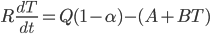
 with equilibrium solution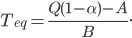

This equilibrium is stable with eigenvalue (recall ).

What if the earth’s albedo was not ? Remember, albedo of ice is , so changing ratios of ice to land to water change overall albedo.

Next step: zonal energy balance models.

We need to look at energy coming in to our planet, whose axis is tilted in space. We want to model with continuous variables like y, the sine of latitude, which gives us our location between the equator and the pole. Then we can make other parameters a function of y. We'll take into account a few more factors than previously.

Heat imbalance = insolation - reflection - reemission - transport

Let's work through these terms.

Transport: we’re going to have the gulf stream, wind, storms, movement through the atmosphere. That is transport. We can model transport by diffusion (want to be like everyone else around us) or we can simply “relax to the global average.”

Reemission includes effects of greenhouse gases. Grave & North, 1993 paper — outgoing longwave radiation detected via satellite. Surface temperature is x, OLR is y. Easiest thing to do is fit a straight line and we use those numbers for A and B as OLR = A+BT.

Reflection: NASA data about albedo. Surface albedo plotted against latitude. Albedo pretty low over continents. So we might as well model albedo with a step function depending on terrain.

Insolation: The rays of light at northern latitudes are coming in at an oblique angle, while nearer the equator we have more direct sunlight. McGehee and Lehman, 2012, give a picture of how insolation is distributed as a function of (find a calculus exercise for this! Integral under the curve is one of course.)

Insolation is also affected by eccentricity (how ellipsoidal our orbit around the sun is) and obliquity (tilt of planet) and precession (our axis wobbles). These have real effects!

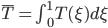
Budyko 1969 (and Tung 2007) came up with something like

R is planetary heat capacity. Function is distribution function (for instance, like in McGehee and Lehman). is temperature. The albedo at given that the ice line is at is . , and so the term represents linear heat transport given by this "relaxation to global average." is around and is picked to fit the data. are the OLR parameters, and and should encapsulate earth orbital components.

Budyko Zonal EBM: there are some great animations here, but I don't know how to do them yet without MATLAB.

Add in albedo feedback

Next add in ice albedo feedback. Warmer climate -> less snow and ice -> more sunlight absorbed by land and sea -> warmer climate. Colder climate -> more ice and snow -> less sunlight absorbed by land and sea -> colder climate. Why aren’t we burning up or freezing into a snowball? What about our model is wrong?

We need to evolve the ice cap boundary! That is, we need to evolve . This changes how much surface ice there is and thus changes the albedo dynamically. Two assumptions:

1. Ice forms or melts at a much slower rate than temperature changes.
2. At the ice line, there’s a critical temperature above which ice will melt and below which ice will form.

What would this equation look like?

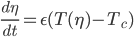
The epsilon makes sure this is a slow-moving ice line.

Consequences:

1. The temperature quickly approaches equilibrium while the ice line moves slowly.
2. The dynamics of the ice line when the temperature profile is near is approximately

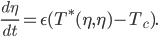
That brings us to a one-dimensional equation. Can draw as output of . Get two equilibria: one source, one sink. According to this model, we’ll always have a bit of ice and never be a snowball earth. So Budyko EBM with a slow moving ice line gives us something really useful.

Interesting questions to be addressed later

1. effects of increasing greenhouse gases? Jim Walsh
2. variable insolation, eg Milankovitch cycle? Dick McGehee
3. what climate states can this model predict? Anna Barry

Jody Sorenson asks, what do we need to add to the model in order to account for ice age - small ice cap - ice age - ice cap cycle? Esther replies: good question! Several answers... and we will address them later 🙂